Learn how to handle spatial data analysis using R.
Spatial
R
Author
Isaac Ajao
Published
January 14, 2026
In this blog, I will demonstrate how to perform spatial data analysis using R, focusing on techniques for exploring and modeling spatial relationships in your data. You’ll learn how to handle spatial data, visualize spatial patterns, and apply spatial econometric models to gain deeper insights into spatial dependencies.
Case study: Reading Culture Among Higher Education Students in Southwestern Nigeria.
Introduction
Spatial econometrics is a branch of econometrics that deals with the modeling and analysis of spatially dependent data. In traditional econometrics, observations are often assumed to be independent of each other, but in spatial econometrics, it is recognized that observations from nearby locations can influence each other, creating spatial dependence.
This analysis incorporates spatial relationships into models through spatial weights matrices, which define the structure of these dependencies. Two common forms of spatial dependence are spatial lag (where the value of a variable in one location depends on the values of the same variable in nearby locations) and spatial error (where errors in one location are correlated with errors in nearby locations).
Spatial econometrics is especially useful in fields like regional economics, real estate, environmental studies, and geography, where spatial factors significantly impact the relationships being studied. It allows for more accurate modeling and understanding of phenomena such as housing prices, land use, and even the spread of diseases, taking into account the spatial proximity of observations.
Load the necessary libraries
library(sf)
Linking to GEOS 3.12.1, GDAL 3.8.4, PROJ 9.3.1; sf_use_s2() is TRUE
library(spdep)
Loading required package: spData
To access larger datasets in this package, install the spDataLarge
package with: `install.packages('spDataLarge',
repos='https://nowosad.github.io/drat/', type='source')`
library(splm)library(spatialreg)
Loading required package: Matrix
Attaching package: 'spatialreg'
The following objects are masked from 'package:spdep':

    get.ClusterOption, get.coresOption, get.mcOption,
    get.VerboseOption, get.ZeroPolicyOption, set.ClusterOption,
    set.coresOption, set.mcOption, set.VerboseOption,
    set.ZeroPolicyOption
library(sp)library(stargazer)
Please cite as:
Hlavac, Marek (2022). stargazer: Well-Formatted Regression and Summary Statistics Tables.
R package version 5.2.3. https://CRAN.R-project.org/package=stargazer
      ID_0         ISO               NAME_0               ID_1
 Min.   :163   Length:38          Length:38          Min.   : 1.00
 1st Qu.:163   Class :character   Class :character   1st Qu.:10.25
 Median :163   Mode  :character   Mode  :character   Median :19.50
 Mean   :163                                         Mean   :19.50
 3rd Qu.:163                                         3rd Qu.:28.75
 Max.   :163                                         Max.   :38.00
    NAME_1             TYPE_1           ENGTYPE_1          NL_NAME_1
 Length:38          Length:38          Length:38          Length:38
 Class :character   Class :character   Class :character   Class :character
 Mode  :character   Mode  :character   Mode  :character   Mode  :character


  VARNAME_1           reading_hr      books_read          cgpa
 Length:38          Min.   :0.000   Min.   : 0.000   Min.   :0.000
 Class :character   1st Qu.:2.250   1st Qu.: 3.000   1st Qu.:2.962
 Mode  :character   Median :2.735   Median : 4.000   Median :3.085
                    Mean   :2.753   Mean   : 4.395   Mean   :2.904
                    3rd Qu.:3.060   3rd Qu.: 5.000   3rd Qu.:3.413
                    Max.   :6.000   Max.   :12.000   Max.   :3.930
   love_readi      met_standa      finis_book         long
 Min.   :0.000   Min.   :0.000   Min.   :0.000   Min.   : 3.474
 1st Qu.:2.000   1st Qu.:2.000   1st Qu.:2.000   1st Qu.: 5.672
 Median :2.000   Median :2.000   Median :2.000   Median : 7.314
 Mean   :1.974   Mean   :1.947   Mean   :1.895   Mean   : 7.556
 3rd Qu.:2.000   3rd Qu.:2.000   3rd Qu.:2.000   3rd Qu.: 8.705
 Max.   :3.000   Max.   :3.000   Max.   :3.000   Max.   :14.450
      lat                  geometry
 Min.   : 4.772   MULTIPOLYGON :38
 1st Qu.: 6.525   epsg:4326    : 0
 Median : 8.089   +proj=long...: 0
 Mean   : 8.597
 3rd Qu.:10.686
 Max.   :13.110
head(reading)
Simple feature collection with 6 features and 17 fields
Geometry type: MULTIPOLYGON
Dimension:     XY
Bounding box:  xmin: 5.376527 ymin: 4.270418 xmax: 13.72793 ymax: 12.5025
Geodetic CRS:  WGS 84
  ID_0 ISO  NAME_0 ID_1    NAME_1 TYPE_1 ENGTYPE_1 NL_NAME_1 VARNAME_1
1  163 NGA Nigeria    1      Abia  State     State      <NA>      <NA>
2  163 NGA Nigeria    2   Adamawa  State     State      <NA>      <NA>
3  163 NGA Nigeria    3 Akwa Ibom  State     State      <NA>      <NA>
4  163 NGA Nigeria    4   Anambra  State     State      <NA>      <NA>
5  163 NGA Nigeria    5    Bauchi  State     State      <NA>      <NA>
6  163 NGA Nigeria    6   Bayelsa  State     State      <NA>      <NA>
  reading_hr books_read cgpa love_readi met_standa finis_book      long
1       3.06          4 3.01          2          2          2  7.524533
2       2.06          5 2.69          3          2          2 12.400776
3       2.20          3 3.52          2          2          2  7.846249
4       2.66          4 3.43          2          2          2  6.935840
5       2.75          4 3.13          2          3          2  9.985480
6       2.25          5 2.76          3          2          2  6.072448
        lat                       geometry
1  5.456715 MULTIPOLYGON (((7.508013 6....
2  9.324338 MULTIPOLYGON (((13.72386 10...
3  4.907001 MULTIPOLYGON (((7.610695 4....
4  6.227947 MULTIPOLYGON (((6.915181 6....
5 10.784808 MULTIPOLYGON (((10.73445 12...
6  4.772090 MULTIPOLYGON (((6.440416 4....
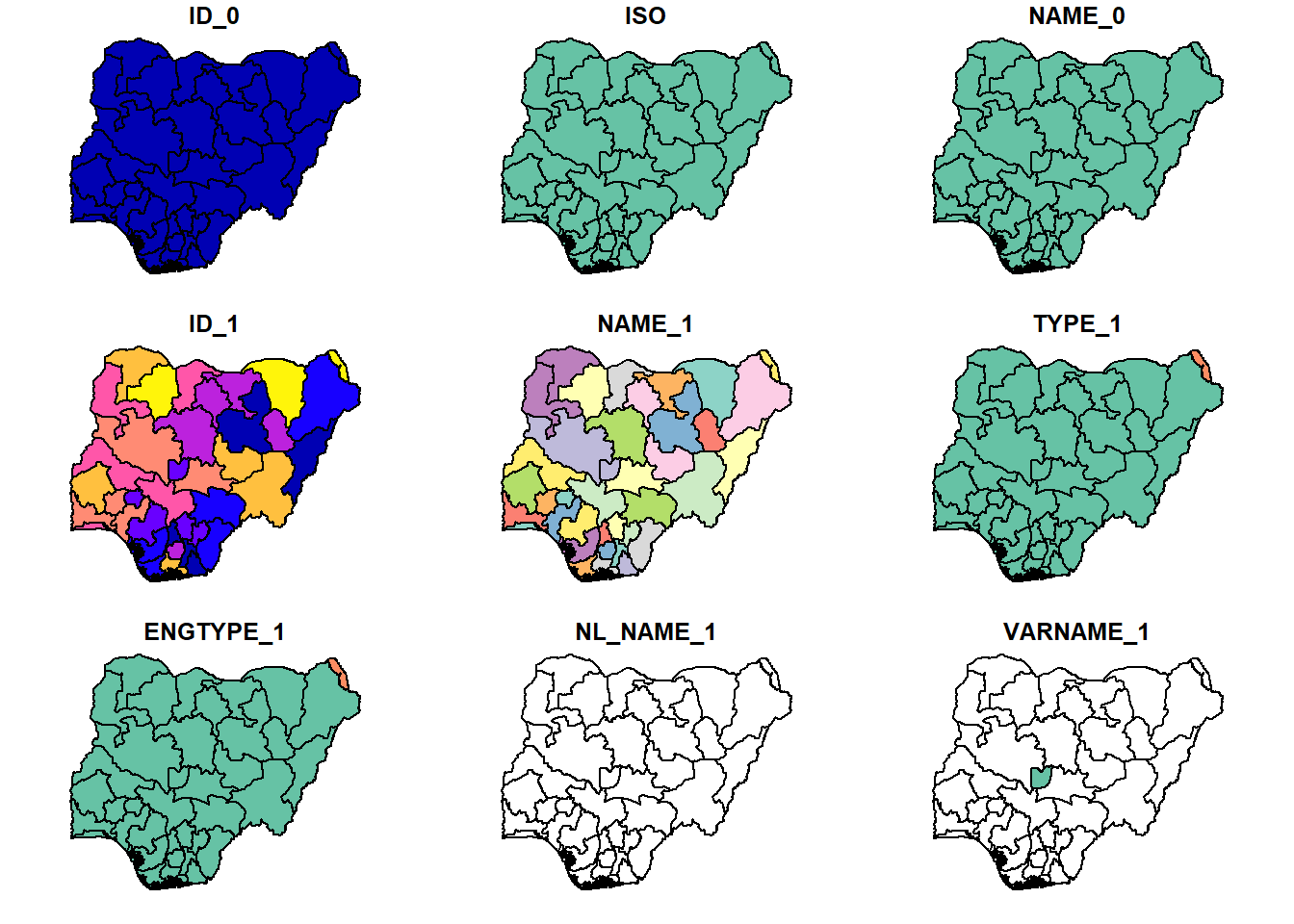
plot(reading)
Warning: plotting the first 9 out of 17 attributes; use max.plot = 17 to plot
all
class(reading)
[1] "sf" "data.frame"
str(reading)
Classes 'sf' and 'data.frame':  38 obs. of  18 variables:
 $ ID_0      : num  163 163 163 163 163 163 163 163 163 163 ...
 $ ISO       : chr  "NGA" "NGA" "NGA" "NGA" ...
 $ NAME_0    : chr  "Nigeria" "Nigeria" "Nigeria" "Nigeria" ...
 $ ID_1      : num  1 2 3 4 5 6 7 8 9 10 ...
 $ NAME_1    : chr  "Abia" "Adamawa" "Akwa Ibom" "Anambra" ...
 $ TYPE_1    : chr  "State" "State" "State" "State" ...
 $ ENGTYPE_1 : chr  "State" "State" "State" "State" ...
 $ NL_NAME_1 : chr  NA NA NA NA ...
 $ VARNAME_1 : chr  NA NA NA NA ...
 $ reading_hr: num  3.06 2.06 2.2 2.66 2.75 2.25 3.06 2 3.5 2.42 ...
 $ books_read: num  4 5 3 4 4 5 5 2 3 3 ...
 $ cgpa      : num  3.01 2.69 3.52 3.43 3.13 2.76 3.13 2 3.51 3.5 ...
 $ love_readi: num  2 3 2 2 2 3 2 1 2 2 ...
 $ met_standa: num  2 2 2 2 3 2 2 2 2 2 ...
 $ finis_book: num  2 2 2 2 2 2 2 1 2 2 ...
 $ long      : num  7.52 12.4 7.85 6.94 9.99 ...
 $ lat       : num  5.46 9.32 4.91 6.23 10.78 ...
 $ geometry  :sfc_MULTIPOLYGON of length 38; first list element: List of 1
  ..$ :List of 1
  .. ..$ : num [1:302, 1:2] 7.51 7.52 7.53 7.53 7.53 ...
  ..- attr(*, "class")= chr [1:3] "XY" "MULTIPOLYGON" "sfg"
 - attr(*, "sf_column")= chr "geometry"
 - attr(*, "agr")= Factor w/ 3 levels "constant","aggregate",..: NA NA NA NA NA NA NA NA NA NA ...
  ..- attr(*, "names")= chr [1:17] "ID_0" "ISO" "NAME_0" "ID_1" ...
st_is_longlat(reading) # checking whether the geographical coordinates have been
[1] TRUE
#projected (the result TRUE means not)

st_crs(reading) #checking which mapping was applied
Reading layer `reading_cultre' from data source
  `C:\Users\user\Desktop\softdataconsult.github.io\blog\posts\spatial\reading_cultre.shp'
  using driver `ESRI Shapefile'
Simple feature collection with 38 features and 17 fields
Geometry type: MULTIPOLYGON
Dimension:     XY
Bounding box:  xmin: 2.668431 ymin: 4.270418 xmax: 14.67642 ymax: 13.89201
Geodetic CRS:  WGS 84
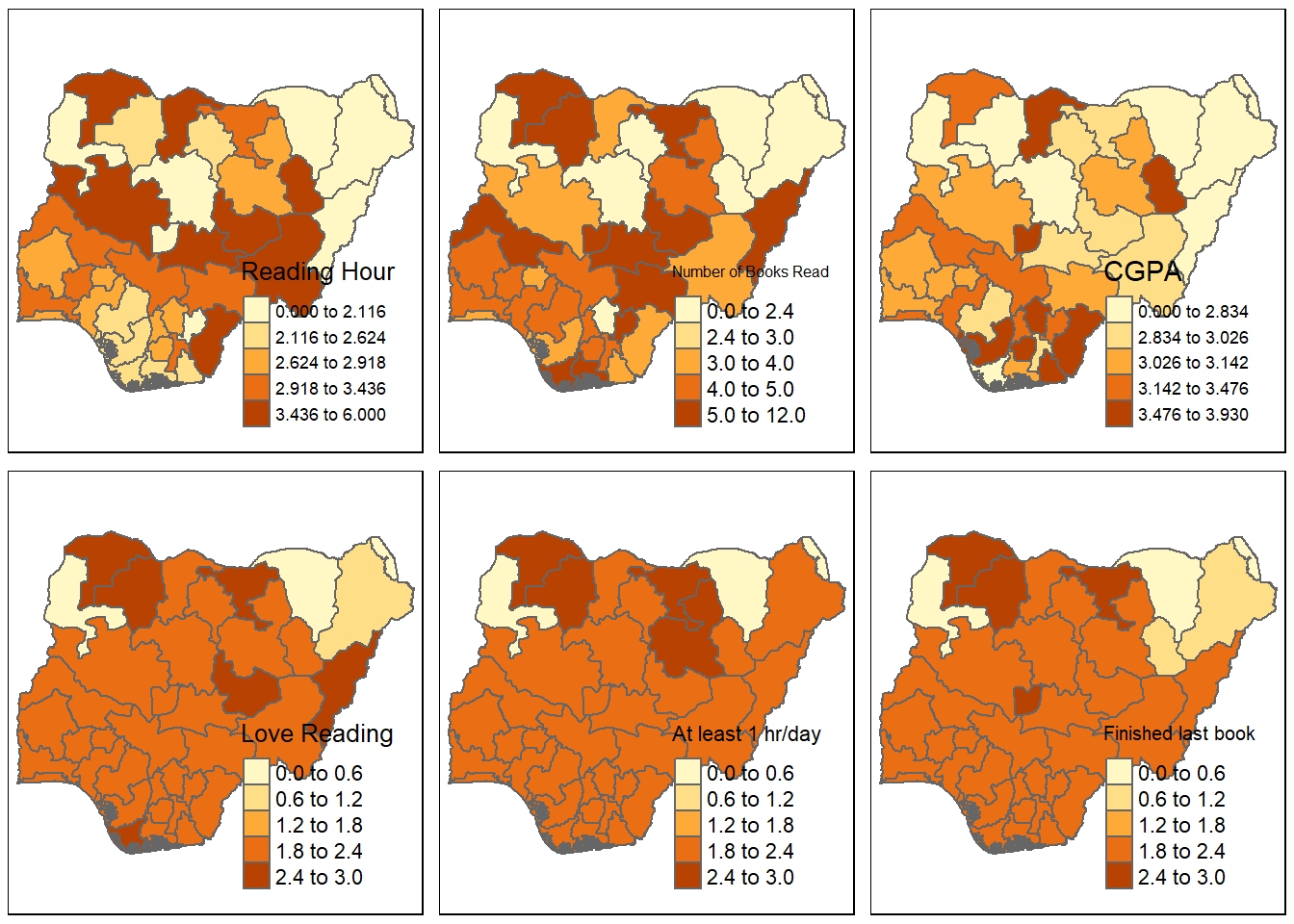
# Set up a 2x3 layout with tmaptm_layout <-tm_layout(title =c("Reading Hour", "Books Read", "CGPA", "Love Reading", "At least 1 hr/day", "Finished last book"),frame =FALSE,asp =0) # Set aspect ratio to 0 for individual map customization# Plot the first maptm1 <-tm_shape(reading_sf) +tm_borders() +tm_fill("reading_hr", title ="Reading Hour", style ="quantile")# Plot the second maptm2 <-tm_shape(reading_sf) +tm_borders() +tm_fill("books_read", title ="Number of Books Read", style ="quantile")# Plot the third maptm3 <-tm_shape(reading_sf) +tm_borders() +tm_fill("cgpa", title ="CGPA", style ="quantile")# Plot the fourth maptm4 <-tm_shape(reading_sf) +tm_borders() +tm_fill("love_readi", title ="Love Reading", style ="quantile")# Plot the fifth maptm5 <-tm_shape(reading_sf) +tm_borders() +tm_fill("met_standa", title ="At least 1 hr/day", style ="quantile")# Plot the sixth maptm6 <-tm_shape(reading_sf) +tm_borders() +tm_fill("finis_book", title ="Finished last book", style ="quantile")# Display the maps in a 2x3 layouttmap_arrange(list(tm1, tm2, tm3, tm4, tm5, tm6), layout = tm_layout)
Legend labels were too wide. The labels have been resized to 0.55, 0.55, 0.55, 0.55, 0.55. Increase legend.width (argument of tm_layout) to make the legend wider and therefore the labels larger.
Legend labels were too wide. The labels have been resized to 0.55, 0.55, 0.55, 0.55, 0.55. Increase legend.width (argument of tm_layout) to make the legend wider and therefore the labels larger.
# read the data from excel for other analysisreading_data <-read.csv("reading_culture_coordinates.csv")
#define our regression equation so we don't have to type it each timereg.eq1=reading_hr ~ books_read + cgpa + love_readi + met_standa + finis_bookreg1=lm(reg.eq1,data=reading)
Warning in mat2listw(matrix(rbinom(nrow(reading_data)^2, 1, 0.2),
nrow(reading_data))): style is M (missing); style should be set to a valid
value
listw
Characteristics of weights list object:
Neighbour list object:
Number of regions: 38
Number of nonzero links: 255
Percentage nonzero weights: 17.65928
Average number of links: 6.710526
Non-symmetric neighbours list

Weights style: M
Weights constants summary:
   n   nn  S0  S1   S2
M 38 1444 255 310 7264
lm.morantest
lm.morantest(reg1, listw )
    Global Moran I for regression residuals

data:
model: lm(formula = reg.eq1, data = reading)
weights: listw

Moran I statistic standard deviate = 2.4478, p-value = 0.007186
alternative hypothesis: greater
sample estimates:
Observed Moran I      Expectation         Variance
     0.097317729     -0.034432679      0.002896984
Let’s run the Four simplest models: OLS, SLX, Lag Y, and Lag Error
Call:
lm(formula = reg.eq1, data = reading)

Residuals:
    Min      1Q  Median      3Q     Max
-1.5992 -0.5211 -0.1218  0.1665  3.3228

Coefficients:
            Estimate Std. Error t value Pr(>|t|)
(Intercept)  0.07031    0.51720   0.136   0.8927
books_read   0.07339    0.08281   0.886   0.3821
cgpa         0.76432    0.33255   2.298   0.0282 *
love_readi   0.30082    0.49804   0.604   0.5501
met_standa   0.53481    0.57056   0.937   0.3556
finis_book  -0.78873    0.61250  -1.288   0.2071
---
Signif. codes:  0 '***' 0.001 '**' 0.01 '*' 0.05 '.' 0.1 ' ' 1

Residual standard error: 0.9277 on 32 degrees of freedom
Multiple R-squared:  0.4904,    Adjusted R-squared:  0.4108
F-statistic: 6.159 on 5 and 32 DF,  p-value: 0.000419
summary(reg1b)
Call:
lm(formula = reading_hr ~ books_read + cgpa + love_readi + met_standa +
    finis_book, data = reading)

Residuals:
    Min      1Q  Median      3Q     Max
-1.5992 -0.5211 -0.1218  0.1665  3.3228

Coefficients:
            Estimate Std. Error t value Pr(>|t|)
(Intercept)  0.07031    0.51720   0.136   0.8927
books_read   0.07339    0.08281   0.886   0.3821
cgpa         0.76432    0.33255   2.298   0.0282 *
love_readi   0.30082    0.49804   0.604   0.5501
met_standa   0.53481    0.57056   0.937   0.3556
finis_book  -0.78873    0.61250  -1.288   0.2071
---
Signif. codes:  0 '***' 0.001 '**' 0.01 '*' 0.05 '.' 0.1 ' ' 1

Residual standard error: 0.9277 on 32 degrees of freedom
Multiple R-squared:  0.4904,    Adjusted R-squared:  0.4108
F-statistic: 6.159 on 5 and 32 DF,  p-value: 0.000419
lm.morantest(reg1,listw)
    Global Moran I for regression residuals

data:
model: lm(formula = reg.eq1, data = reading)
weights: listw

Moran I statistic standard deviate = 2.4478, p-value = 0.007186
alternative hypothesis: greater
sample estimates:
Observed Moran I      Expectation         Variance
     0.097317729     -0.034432679      0.002896984
Please update scripts to use lm.RStests in place of lm.LMtests
Warning in lm.RStests(model = model, listw = listw, zero.policy = zero.policy,
: Spatial weights matrix not row standardized
    Rao's score (a.k.a Lagrange multiplier) diagnostics for spatial
    dependence

data:
model: lm(formula = reg.eq1, data = reading)
test weights: listw

RSerr = 1.9866, df = 1, p-value = 0.1587


    Rao's score (a.k.a Lagrange multiplier) diagnostics for spatial
    dependence

data:
model: lm(formula = reg.eq1, data = reading)
test weights: listw

RSlag = 0.047814, df = 1, p-value = 0.8269


    Rao's score (a.k.a Lagrange multiplier) diagnostics for spatial
    dependence

data:
model: lm(formula = reg.eq1, data = reading)
test weights: listw

adjRSerr = 2.5486, df = 1, p-value = 0.1104


    Rao's score (a.k.a Lagrange multiplier) diagnostics for spatial
    dependence

data:
model: lm(formula = reg.eq1, data = reading)
test weights: listw

adjRSlag = 0.6098, df = 1, p-value = 0.4349


    Rao's score (a.k.a Lagrange multiplier) diagnostics for spatial
    dependence

data:
model: lm(formula = reg.eq1, data = reading)
test weights: listw

SARMA = 2.5964, df = 2, p-value = 0.273
SLX (Spatial Lag Model with Exogenous Variables)
# Assuming your data is named 'your_data'# Load required packageslibrary(spatialreg)# Create an 'sf' object with the spatial coordinatesreading_sf_data <-st_as_sf(reading_data, coords =c("long", "lat"))# Create a spatial weights matrix (queen contiguity)listw <-mat2listw(matrix(rbinom(nrow(reading_data)^2, 1, 0.2), nrow(reading_data)))
Warning in mat2listw(matrix(rbinom(nrow(reading_data)^2, 1, 0.2),
nrow(reading_data))): style is M (missing); style should be set to a valid
value
Do you enjoy my blog? Subscribe here to get notifications and updates (it's absolutely free!):
Source Code
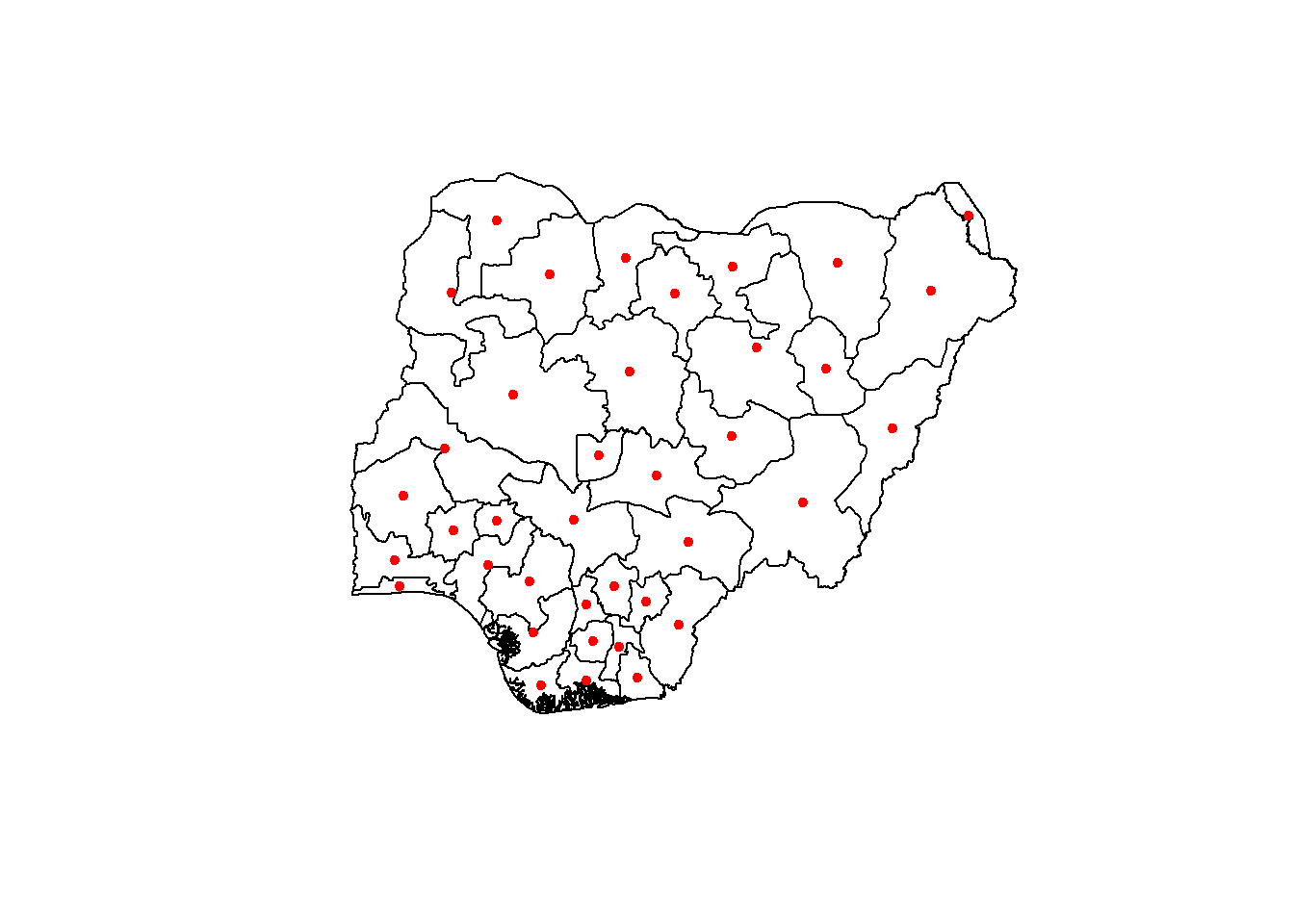
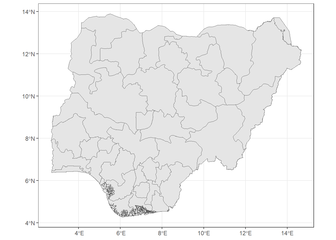
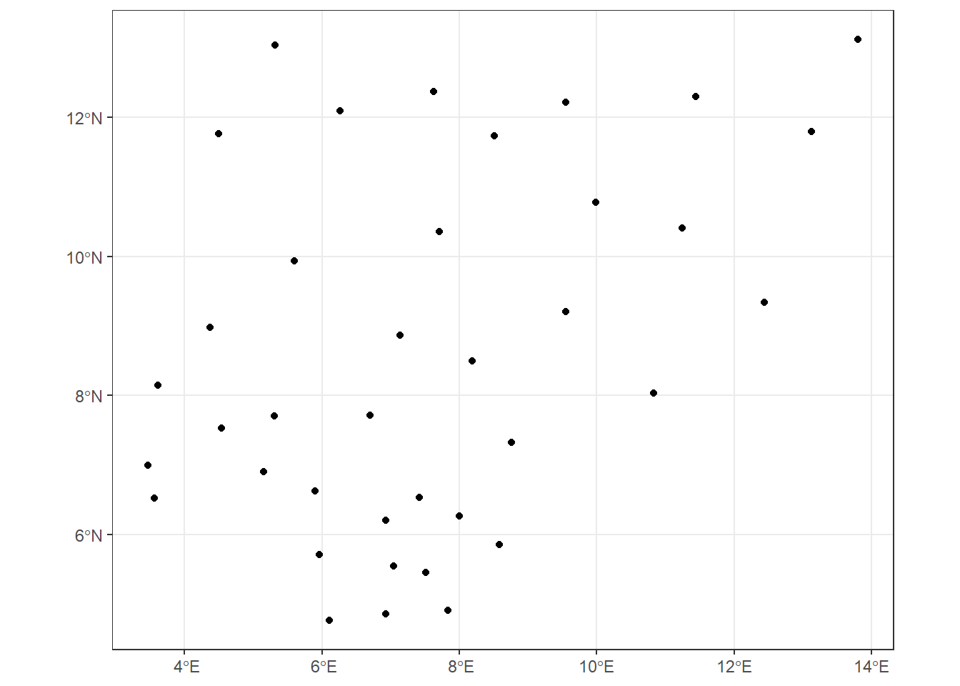
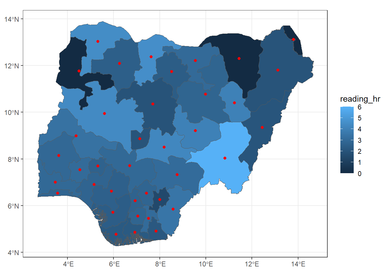
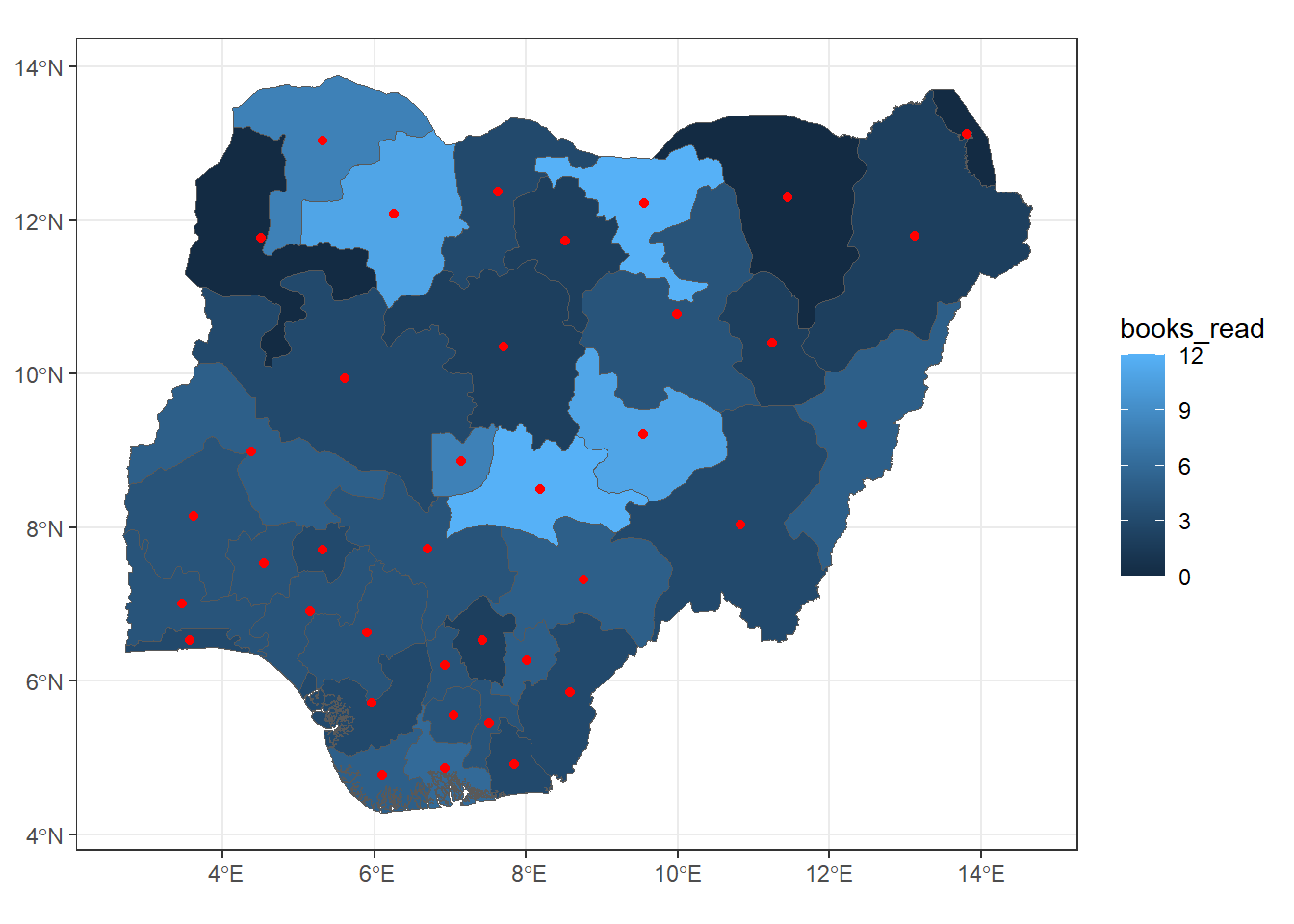
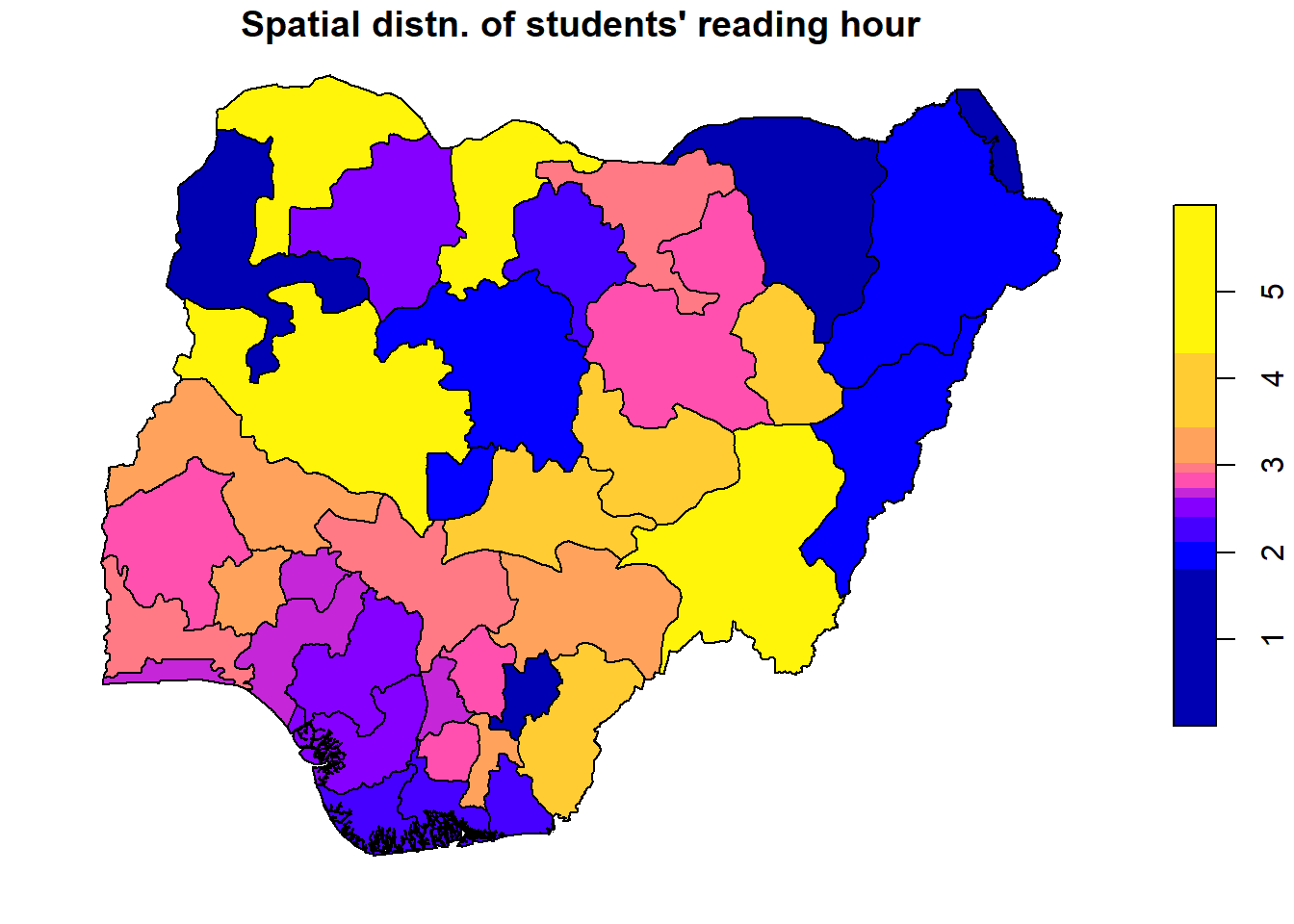
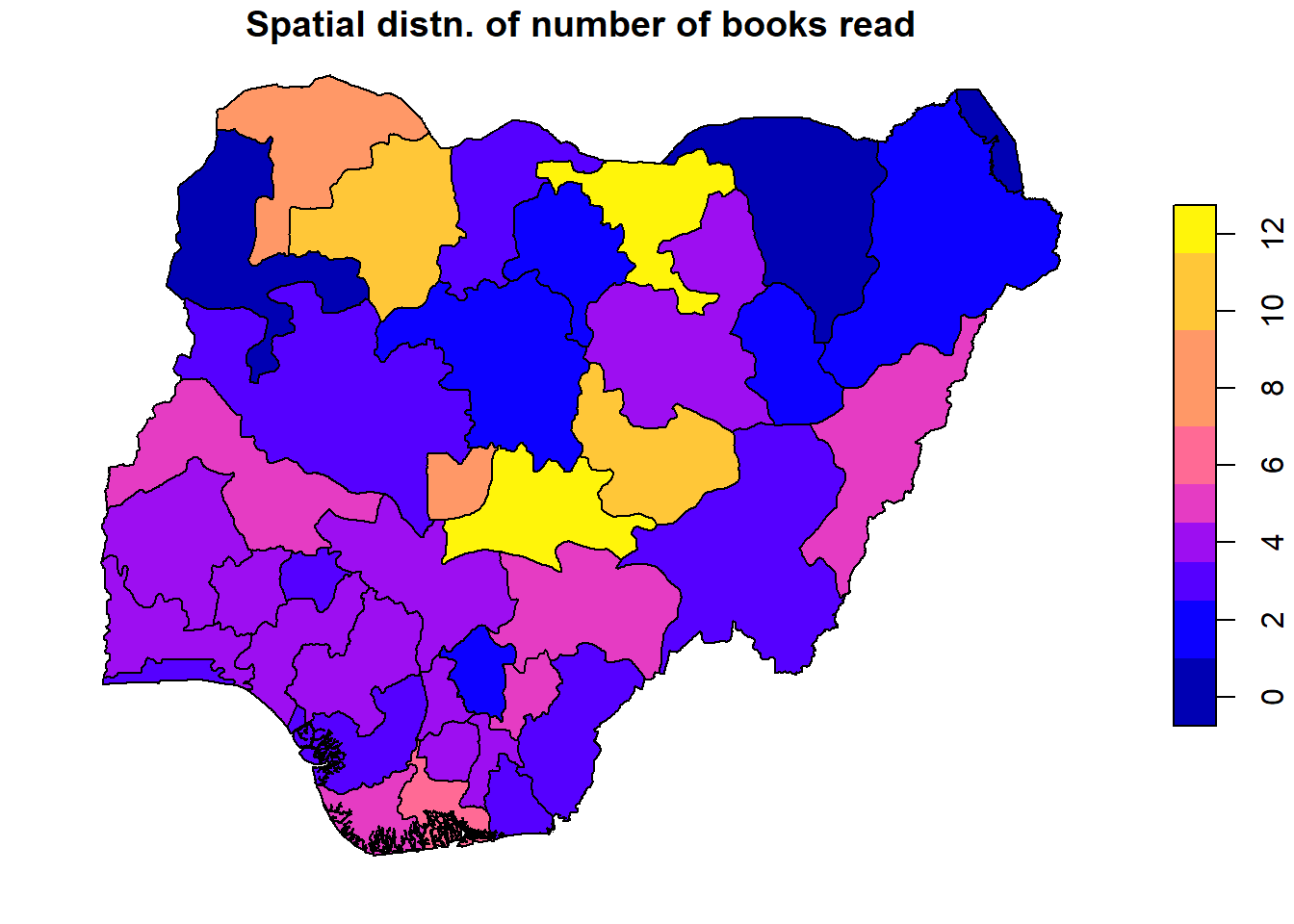
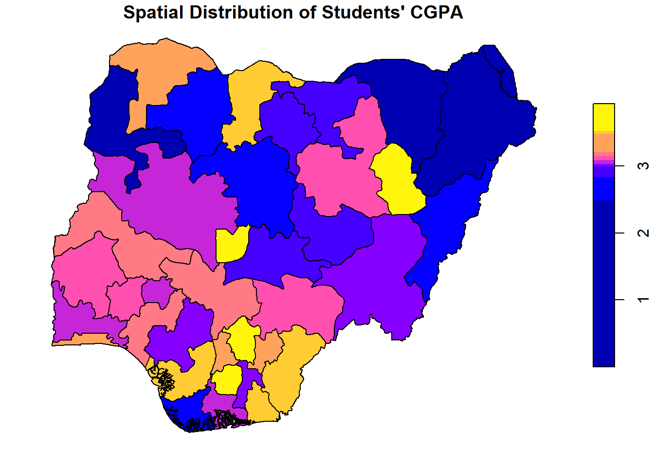
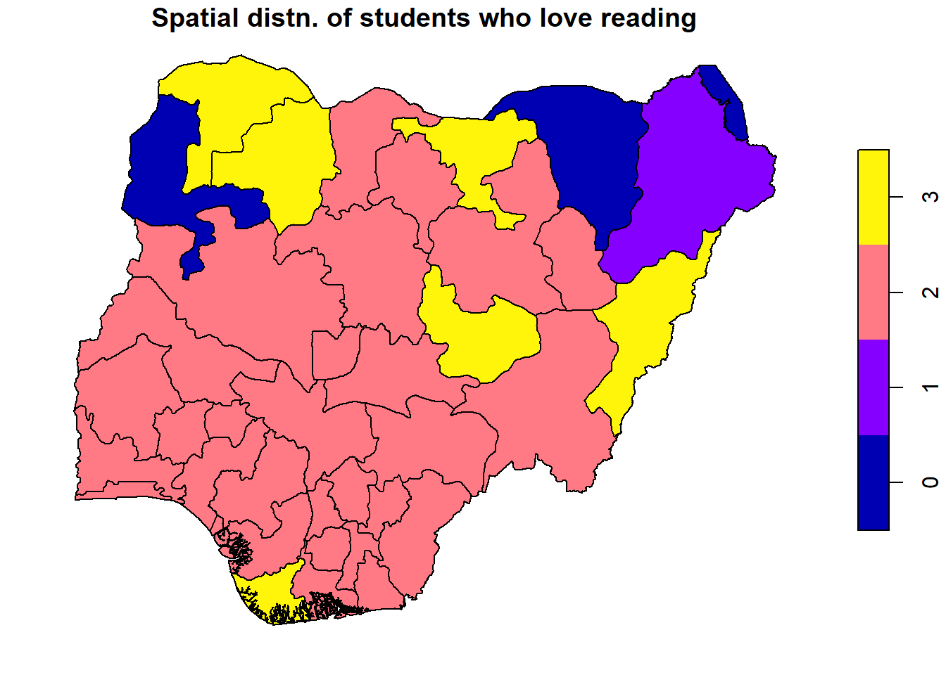
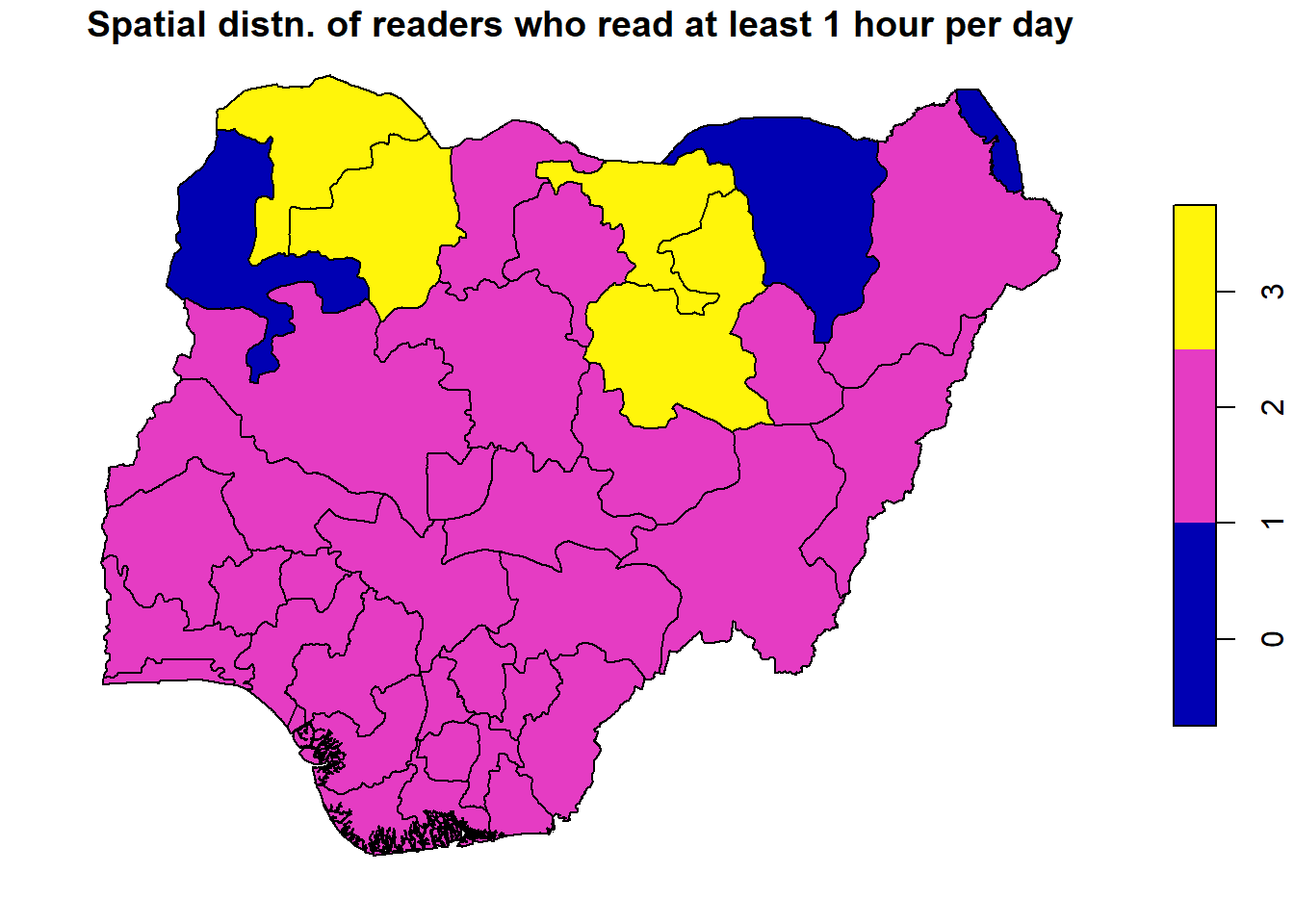
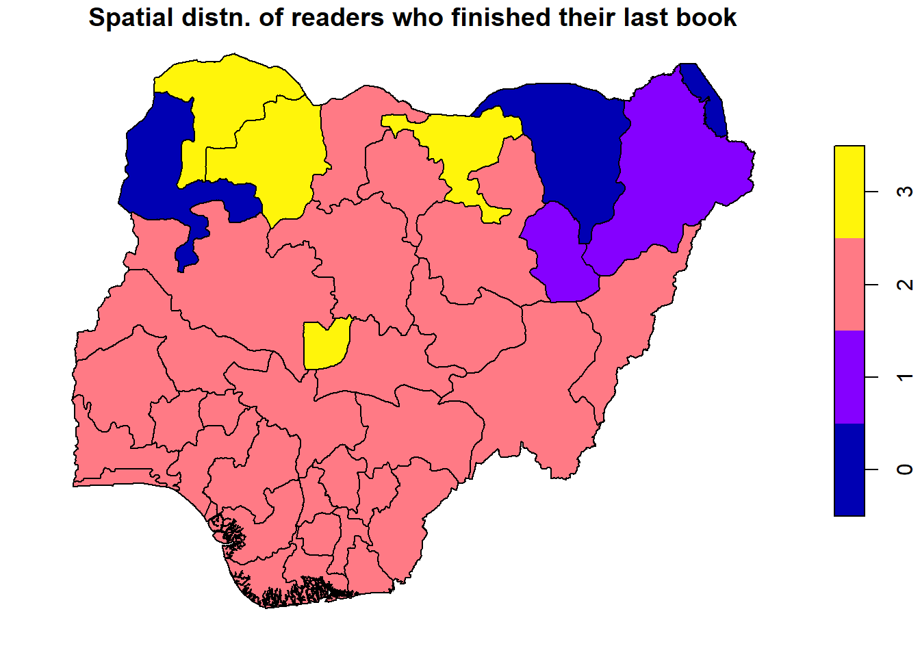
---title: "Spatial Econometrics Data Analysis"description: | Learn how to handle spatial data analysis using R.date: todayauthor: "Isaac Ajao"#date: "2024-10-06"categories: [Spatial, R]image: "spatial2.png"---In this blog, I will demonstrate how to perform spatial data analysis using R, focusing on techniques for exploring and modeling spatial relationships in your data. You'll learn how to handle spatial data, visualize spatial patterns, and apply spatial econometric models to gain deeper insights into spatial dependencies. **Case study:** Reading Culture Among Higher Education Students in Southwestern Nigeria.### Introduction Spatial econometrics is a branch of econometrics that deals with the modeling and analysis of spatially dependent data. In traditional econometrics, observations are often assumed to be independent of each other, but in spatial econometrics, it is recognized that observations from nearby locations can influence each other, creating spatial dependence.This analysis incorporates spatial relationships into models through spatial weights matrices, which define the structure of these dependencies. Two commonforms of spatial dependence are spatial lag (where the value of a variable in one location depends on the values of the same variable in nearby locations) and spatial error (where errors in one location are correlated with errors in nearby locations).Spatial econometrics is especially useful in fields like regional economics, real estate, environmental studies, and geography, where spatial factors significantly impact the relationships being studied. It allows for more accurate modeling and understanding of phenomena such as housing prices, land use, and even the spread of diseases, taking into account the spatial proximity of observations.### Load the necessary libraries```{r}library(sf)library(spdep)library(splm)library(spatialreg)library(sp)library(stargazer)```### Reading the shapefile containing the data```{r}## Reading shape file containing the datareading =st_read("reading_cultre.shp",quiet =TRUE)names(reading) #show variable namessummary(reading)head(reading)plot(reading)``````{r}class(reading)str(reading)st_is_longlat(reading) # checking whether the geographical coordinates have been #projected (the result TRUE means not) st_crs(reading) #checking which mapping was appliedtable(st_is_valid(reading)) # validationreading_sp<-as(reading, "Spatial") class(reading_sp)``````{r}reading_points<-st_cast(reading$geometry, "MULTIPOINT")``````{r}reading_points_count<-sapply(reading_points, length)sum(reading_points_count) # Checking how many vertices are in all counties``````{r}reading_simple<-st_simplify(reading, dTolerance =50)``````{r}reading_simple_points<-st_cast(reading_simple$geometry, "MULTIPOINT")sum(sapply(reading_simple_points, length))``````{r}reading_central<-st_centroid(reading)``````{r}plot(st_geometry(reading))reading_central<-st_centroid(reading)plot(reading_central$geometry, add=TRUE, pch=20, col="red")``````{r}library(ggplot2)ggplot(reading_simple) +geom_sf() +theme_bw() ggplot(reading_central) +geom_sf() +theme_bw() ``````{r}ggplot(reading_simple) +geom_sf(aes(fill = reading_hr)) +theme_bw()``````{r}ggplot() +geom_sf(data=reading_simple, aes(fill=reading_hr)) +geom_sf(data=reading_central, col="red") +theme_bw()``````{r}ggplot() +geom_sf(data=reading_simple, aes(fill=books_read)) +geom_sf(data=reading_central, col="red") +theme_bw()``````{r}reading_sf =st_read("reading_cultre.shp") #shape file earlier createdplot(reading_sf)``````{r}names(reading)reading_sf =st_read("reading_cultre.shp") #shape file earlier createdplot(reading_sf["reading_hr"], main ="Spatial distn. of students' reading hour", breaks ="quantile")``````{r}reading_sf =st_read("reading_cultre.shp") #shape file earlier createdplot(reading_sf["books_read"], main ="Spatial distn. of number of books read", breaks ="quantile")#legend("topright", legend = "books_read", fill = topo.colors(5))``````{r}reading_sf <-st_read("reading_cultre.shp")plot(reading_sf["cgpa"], main ="Spatial Distribution of Students' CGPA", breaks ="quantile")# Add a legend#legend("topright", legend = "CGPA", fill = topo.colors(5))``````{r}reading_sf =st_read("reading_cultre.shp") #shape file earlier createdplot(reading_sf["love_readi"], main ="Spatial distn. of students who love reading", breaks ="quantile")#legend("topright", legend = "Love reading", fill = topo.colors(5))``````{r}reading_sf =st_read("reading_cultre.shp") #shape file earlier createdplot(reading_sf["met_standa"], main ="Spatial distn. of readers who read at least 1 hour per day", breaks ="quantile")``````{r}reading_sf =st_read("reading_cultre.shp") #shape file earlier createdplot(reading_sf["finis_book"], main ="Spatial distn. of readers who finished their last book", breaks ="quantile")```### Six maps in one frame```{r}library(tmap)# Read shapefilereading_sf <-st_read("reading_cultre.shp")# Set up a 2x3 layout with tmaptm_layout <-tm_layout(title =c("Reading Hour", "Books Read", "CGPA", "Love Reading", "At least 1 hr/day", "Finished last book"),frame =FALSE,asp =0) # Set aspect ratio to 0 for individual map customization# Plot the first maptm1 <-tm_shape(reading_sf) +tm_borders() +tm_fill("reading_hr", title ="Reading Hour", style ="quantile")# Plot the second maptm2 <-tm_shape(reading_sf) +tm_borders() +tm_fill("books_read", title ="Number of Books Read", style ="quantile")# Plot the third maptm3 <-tm_shape(reading_sf) +tm_borders() +tm_fill("cgpa", title ="CGPA", style ="quantile")# Plot the fourth maptm4 <-tm_shape(reading_sf) +tm_borders() +tm_fill("love_readi", title ="Love Reading", style ="quantile")# Plot the fifth maptm5 <-tm_shape(reading_sf) +tm_borders() +tm_fill("met_standa", title ="At least 1 hr/day", style ="quantile")# Plot the sixth maptm6 <-tm_shape(reading_sf) +tm_borders() +tm_fill("finis_book", title ="Finished last book", style ="quantile")# Display the maps in a 2x3 layouttmap_arrange(list(tm1, tm2, tm3, tm4, tm5, tm6), layout = tm_layout)``````{r}# read the data from excel for other analysisreading_data <-read.csv("reading_culture_coordinates.csv")``````{r}#define our regression equation so we don't have to type it each timereg.eq1=reading_hr ~ books_read + cgpa + love_readi + met_standa + finis_bookreg1=lm(reg.eq1,data=reading)```### Spatial weights matrix W```{r}# Create a spatial weights matrix (queen contiguity)listw <-mat2listw(matrix(rbinom(nrow(reading_data)^2, 1, 0.2), nrow(reading_data)))listw```### lm.morantest```{r}lm.morantest(reg1, listw )```Let's run the Four simplest models: OLS, SLX, Lag Y, and Lag Error### OLS model```{r}library(spdep)library(spatialreg)reg1=lm(reg.eq1,data=reading)reg1b=lm(reading_hr ~ books_read + cgpa + love_readi + met_standa + finis_book, data=reading)summary(reg1)summary(reg1b)lm.morantest(reg1,listw)#lm.moranplot(reg1,listw1)lm.LMtests(reg1,listw,test=c("LMerr", "LMlag", "RLMerr", "RLMlag", "SARMA"))```### SLX (Spatial Lag Model with Exogenous Variables)```{r}# Assuming your data is named 'your_data'# Load required packageslibrary(spatialreg)# Create an 'sf' object with the spatial coordinatesreading_sf_data <-st_as_sf(reading_data, coords =c("long", "lat"))# Create a spatial weights matrix (queen contiguity)listw <-mat2listw(matrix(rbinom(nrow(reading_data)^2, 1, 0.2), nrow(reading_data)))```